GINsim Documentation
Introduction
GINsim (Gene Interaction Network simulation) is a computer tool for the modeling and simulation of genetic regulatory networks.
Recent developments in functional genomics have generated large amounts of data on gene expression and on the underlying regulatory mechanisms. This has resulted in the progressive mapping of complex regulatory networks. As these networks usually include numerous intertwined feedback circuits, gaining an understanding of their spatio-temporal behaviour defies the intuition of the biologists. In this respect, formal modelling and simulation tools become a necessary complement to experimental tools. As precise information on molecular mechanisms and the values of kinetic parameters are currently difficult to establish, qualitative methods offer a highly attractive approach to model and analyse essential properties of genetic regulatory networks. General information on modelling and analysis of genetic regulatory networks can be found in the following review 1.
GINsim consists of a simulator of qualitative models of genetic regulatory networks based on a discrete, logical formalism.
GINsim allows the user to specify a model of a genetic regulatory network in terms of asynchronous, multivalued logical functions, and to simulate and/or analyse its qualitative dynamical behaviour 2.
GUI
Welcome dialog
Upon launch, GINsim will present the Welcome dialog box below.
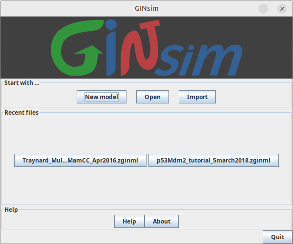
The New model action will create a new Regulatory Graph,
while the Open and Import buttons allow to select an existing file
in a supported format.
The Recent files section allows the quick selection of a previously opened file.
For all these actions, the selected graph will be opened in a Main Window.
Closing this dialog or activating the quit button will stop GINsim.
Info
This dialog is also shown after closing the last window (Ctrl/Cmd-W). Use the Quit (Ctrl/Cmd-Q) action to skip it.
Info
When running GINsim on the command line, it is possible to provide a file to open or to ask for a new model. In this case, the welcome dialog will not be shown. See the run options.
Common quirks
Input nodes
In GINsim, some nodes can be defined as input nodes using a checkbox in the node property panel. These input nodes cannot have any incoming interaction or dynamical rule as they have an implicit rule allowing them to always maintain their current activity level. Before setting a node as input, the modeller must thus remove all existing regulators or rules. Likewise, the input status must be removed before adding any new regulator or rule. To delete a logical formula, select it (without editing it) and use the delete key or the contextual menu.
Unexpected dynamical results
If you obtain unexpected dynamical results (stable states or simulations results), verify successively the structure of the regulatory graph, the maximal activity levels of all components, the thresholds of interactions coming out of multi-valued components and then the dynamical rules. GINsim further provides a tool to compute interaction functionality, which facilitates the identification of inconsistencies between the structure of the regulatory graph and the dynamical rules.
GUI refresh issues
Some refreshing problems may appear after long or complex modeling sessions, saving and restarting GINsim can solve some issues.
Main window
The GINsim window
The main window allows to view a graph, edit its appearance and access to GINsim's main features. This window is divided into three parts:
- the menu and toolbar on the top;
- the graph panel, as the main central part;
- the secondary panel on the bottom.
The main window of GINsim
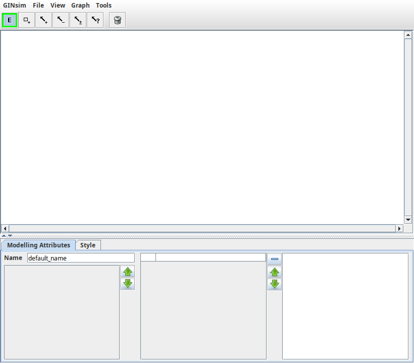
The main window of GINsim, featuring an empty model.
Graph view
see the graph page or merge its content here?
Edit toolbar
The Edit toolbar

The edit toolbar is composed of a few buttons enabling the user to create a new model.
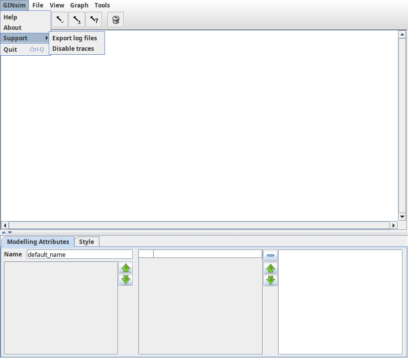
GINsim menu
GINsim menu
Warning
TODO: check and complete
File menu
File menu
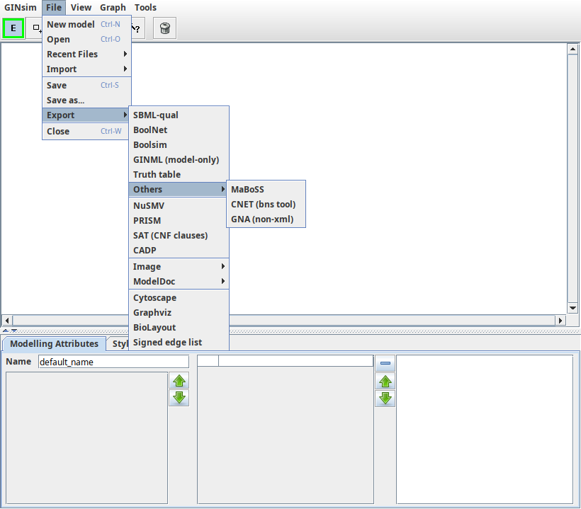
The File menu offers all the classical options to open/save a file, to open/close a window, and to quit the application.
The File menu provides the following options:
- New to create a new graph. This opens a new window unless the current graph is empty.
- Open to load a graph from a file. This opens a new window unless the current graph is empty.
- Recent Files to open a recently used graph. This submenu lists the last opened graphs.
- Merge graph to open a graph and merge it with the current one. This option works only for regulatory graphs.
- Close to close the current graph. If other windows are opened, it will simply close the current one, otherwise it will leave you with an empty window.
- Save/Save as to save the current graph. If the file is new or if the Save as option has been selected, a file selection dialog appears which allows to choose the graphical attributes to save: it is possible to save only the structure of the graph, ignoring all graphical attributes, or to save only the position of nodes. The default is to save all graphical attributes (position, size, color, shape...). The graph is saved in the (XML-based) GINML.
- Save Subgraph to save the current selection as a new graph.
- Export to save the current graph in another format. GINsim can export regulatory and state transition graphs using several generic visualisation formats. These exports only retain the graph structure and visual appearance. The following export formats are available under the File/export submenu: TODO The regulatory graph can additionally be exported into different formats.
- Quit to close all graphs and exit the GINsim application.
Some of these actions New, Open and Save are also available from the toolbar.
The Save dialog
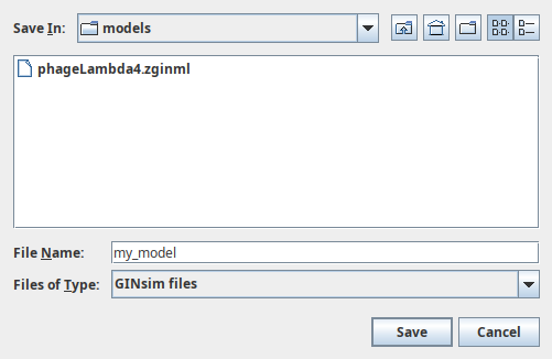
The Java Save dialog allows to browse and create folders, as well as to choose their location. By default, only folders and GINML files are shown; other files can be seen by removing the GINML Files filter. The drop-down list on the right side allows to select the graphical attributes to save. The ExtendedSave checkbox allows to enable or disable extended save (which generates an archive containing the graph and related data).
Info
If the extended save option is selected, the file is saved in an archive (zip file with a .zginml extension) instead of a XML file (with a .ginml extension). This allows to save related data, such as simulation parameters or mutant definitions, along with the model. These files need GINsim 2.3 or later to be opened.
View menu
The View menu
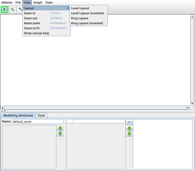
Different actions can be performed from this menu on all types of graph. - Graph layouts; - Level Layout (with or without inversion) - Ring Layout (with or without inversion) - Zoom in/out/reset/fit in window
Graph menu
The Graph menu
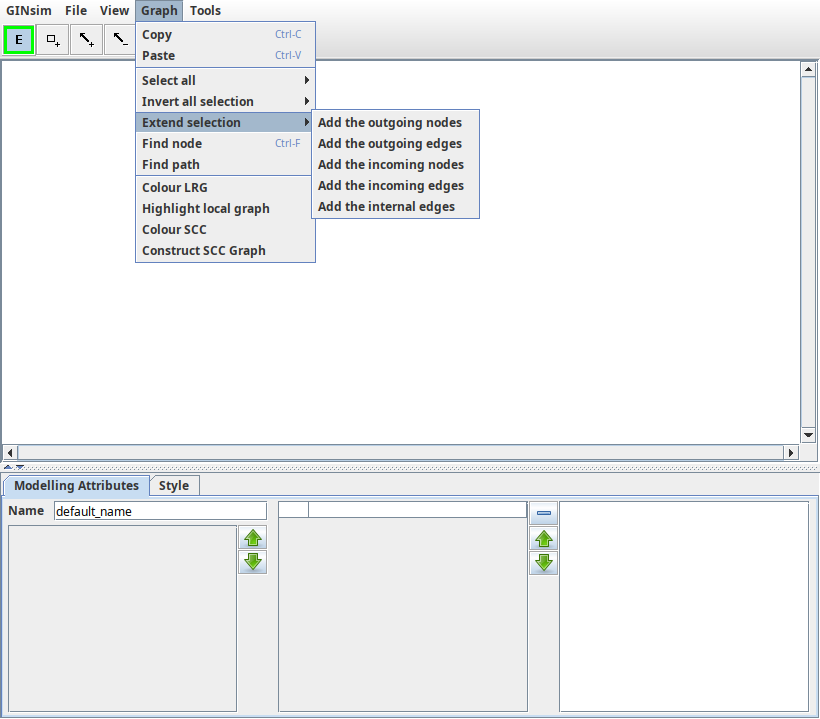
The Graph menu is composed of three sections: copy/paste, selection management, other actions on the logical regulatory graph.
Copy/paste menu section
The edit menu offers classical Copy/Paste entries.
- Regulatory graph elements can be copied and pasted from one GINsim window to another.
- Pasted elements are automatically selected to ease their movement.
- The Copy action does not test selected interactions, it will automatically select ALL interactions between selected genes.
- The identifiers of pasted genes are postfixed to avoid naming conflicts.
- Logical parameters are also copied and cleaned up: logical parameters involving non-copied nodes are suppressed. The resulting graph is consistent but the new parameters may need to be checked.
Warning
Copy/Paste actions are specific to GINsim: copying the graph and pasting it into an external application is not supported. These actions are only available for regulatory graphs.
Selection and search menu section
Warning
TODO: check and complete
Actions menu section
Different actions can be performed from this menu, depending on the type of graph. Individual actions are detailed in the relevant part of this manual. Currently available actions are:
- for all graphs:
- determination of the Strongly Connected Components (SCC) of a graph;
- computation of the local graph; (MISMATCH between tooltip "Compute the local graphs" and menu item "Highlight local graph")
- colouring the regulatory graph, depending on the state of each regulator;
- colouring of the Strongly Connected Components graph.
Warning
TODO: check and complete, is it true for all graphs ?
Tools menu
Warning
TODO: replace this all with a short note and point to the relevant index pages?
The Actions menu
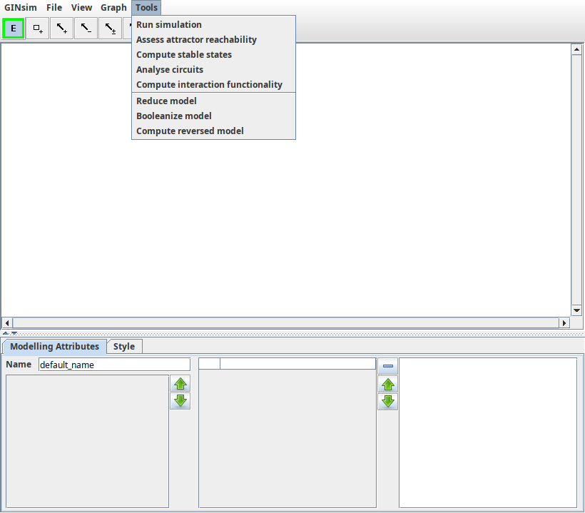
The Action menu for a regulatory graph.
Different actions can be performed from this menu, depending on the type of graph. Individual actions are detailed in the relevant part of this manual. Currently available actions are:
- for regulatory graphs:
- The simulation (i.e., computation of a state transition graph);
- analysis of the Circuit analysis;
- determination of Stable states;
- for state transition graphs:
- path search;
- stg animator graphical path construction (animation);
The secondary panel
The bottom panel allows to edit the items selected in the graph view. It contains two tabs:
- The first tab (called
Modelling Attributesfor regulatory graphs) will change with the type of graph. Panels for the various graph types are described in the corresponding sections. - The
Graphical Attributestab allows to edit the appareance of the selected items. It is described in the graph view page.
Logical Regulatory Graph
Definition
Informally, a Logical Regulatory Graph (LRG) is a directed labelled multigraph representing interactions (the edges) between genes (the nodes). Each interaction involves two genes, the source and the target, becoming active whenever its source reaches a given level.
The activation level of each component is defined by a regulatory function comprising parameters relative to all regulators of this component.
For a more formal definition see 3 or 4.
Structure of the LRG
Regulatory graphs can be interactively modified: components and interactions can be added, edited and removed. The interaction with the graph view is controlled by an editing mode selected through the following buttons available on the toolbar on the top:
Available editing modes for regulatory graphs:
 Default editing mode: allows to select and move objects.
-
 Component insertion mode: when selected, clicking on the graph panel adds a new component.
 -


 Interaction insertion mode: when selected, interactions are added by first
selecting one component and dragging the selection to (the same or) another
component. The interactions must be complemented by the definition of the logical
parameters for the target variable (see below). The four buttons allow to add
different types of interactions: activation, inhibition, dual or undefined.
Interaction insertion mode: when selected, interactions are added by first
selecting one component and dragging the selection to (the same or) another
component. The interactions must be complemented by the definition of the logical
parameters for the target variable (see below). The four buttons allow to add
different types of interactions: activation, inhibition, dual or undefined.  Deletion option: selected items (components or interactions) are deleted.
Info
The terms component and interaction are used throughout this document, but some other terms are sometimes used in their place. Regulatory components (also called nodes) can be of different types. They often denote genes but also proteins, or yet global cellular characteristics such as cell mass. Similarly, interactions often denote transcriptional regulations but can also denote protein phosphorylation, degradation, complex formation, ...
Component order
In GINsim, components are internally ordered. This order has no effect on the regulatory
graph itself, but it has a direct effect on the internal representation of the logical
parameters, with possible effects on (partial) simulation.
The default order follows the node addition chronology, which can be modified
by selecting a (set of) node(s) and using the Up/Down arrows on the left
side of the Modelling Attributes tab.
This change of order will have an effect throughout GINsim, e.g. in the
state transition graph, since the same order is used in the states names.
Changing component order
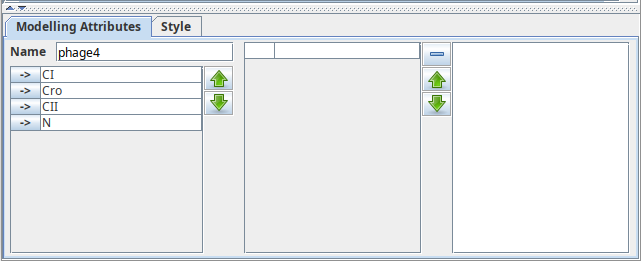
The left part of the Modelling Attributes tab of a regulatory graph lists all components of the model and allows to modify their order. The "up" and "down" buttons move selected components in the list.
Info
The selection of several components, can be achieved (like in all lists) by using the Ctrl key (apple/Cmd key on Mac OS X) or Shift key, while selecting the nodes.
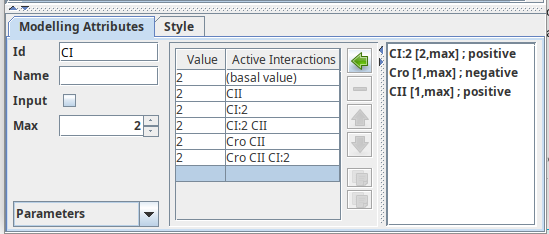
Component attributes
When a single component is selected, the Modelling Attributes
tab allows to define its properties:
Id: component's identifier. It appears in the graph and it must be unique.Name: component's long name (optional).Input: mark a component as an input node, i.e., cannot have regulators.Max: the maximal expression level of the component. The default value is 1 (Boolean case). It can be augmented to generate multi-valued components.Logical parameters: define the rules controlling the dynamical evolution of the expression level depending on the active incoming interactions.
Attributes of a component
Properties of the gene Cro, as defined in the lambda4 model.
Info
The Modelling Attributes tab is divided into three parts.
The combobox selection list (bottom left) permits to select :doc:annotations, as well as Dynamical rules.
Interactions
When a single interaction arc is selected, the Modelling Attributes tab allows to define its properties.
Properties of an interaction arc
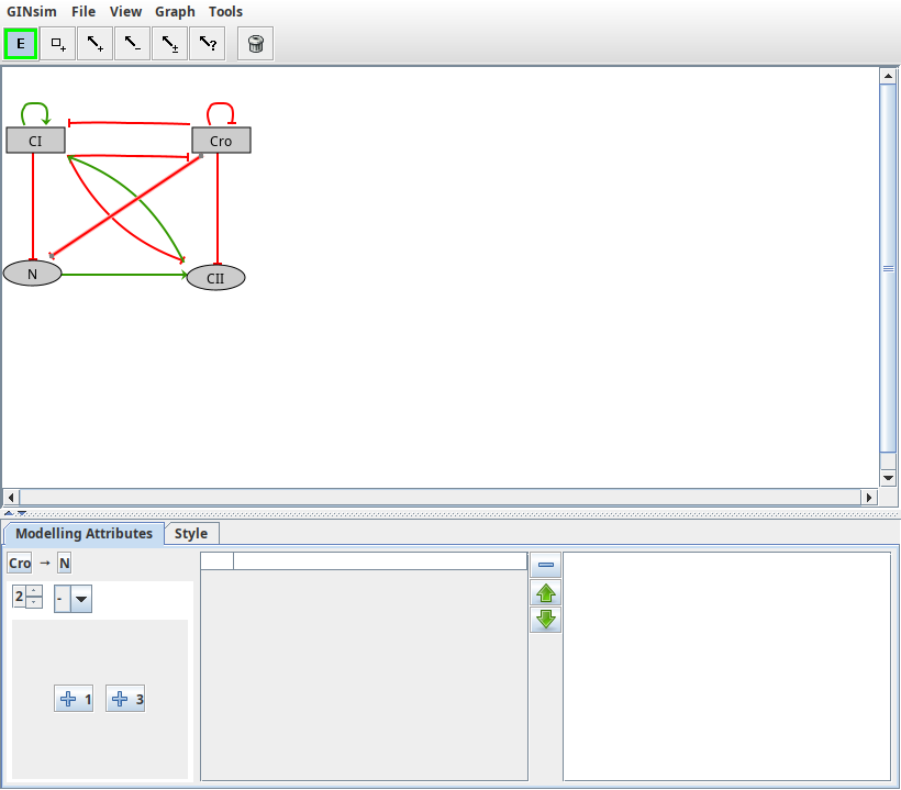
Properties of the Cro-N interaction in the lambda4 model.
Depending on a component's activity level, different effects might occur on another component. These different effects are controlled by the definition of different ranges listed on the left.
- The "+" button creates an additional interaction range.
- The "-" button deletes the selected interaction range.
- Properties of the selected interaction range can be defined:
- Threshold defines the lower bound of the selected interaction range. The interaction becomes active when the activity level of its source component is in this range.
- Sign: each interaction range can be labelled with activation, inhibition, dual or unknown. However, this is only a visual hint, as the real effects of interactions are defined through Dynamical rules.
Model integrity
GINsim keeps the definition of regulatory graphs consistent, which means that:
- When an interaction is deleted, all Dynamical rules in which it was involved are also deleted.
- When the
max valueof a node is decreased, interactions and logical parameters are checked and, if necessary, updated accordingly and silently to avoid inconsistencies.
Since such changes have automatic repercussions on the model parameters and interaction ranges to keep the model valid, keep in mind that you need to double-check parameters after performing such changes.
Checking activation intervals of interactions and the correctness of logical parameters is left to the user as adding more controls generates more annoyances than real help. Invalid logical parameters are highlighted to ease their detection. Keep in mind that a change in the activation-range of one of the interactions can turn a valid logical parameter into an ill-defined one. Parameters involving interactions from the same source with disjoint activity ranges are also ill-defined and thus highlighted for correction.
Dynamical rules
The dynamical behaviour of regulatory components depends on their regulators, but the precise rules governing them must be explicitly defined. In GINsim, these rules can be defined either as logical parameters, or as logical functions. These two alternatives are described below.
Logical parameters
A logical parameter corresponds to a single entry (line) in the truthtable of a component. It is defined by a target activity level and a list of active interactions. By default, interactions not present on the list are implicitly considered to be inactive. This means that in order to a given parameter to be effective, all interactions present on the list must be active, and all interactions not present on the list must be inactive.
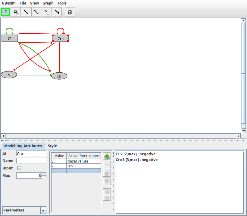
When a component is selected, logical parameters for this component can be
defined in the right part of the Modelling Attribute tab. The panel dedicated
to the definition of logical parameters is divided into three parts:
- On the left, a table lists all defined logical parameters, showing their values and related interactions.
- A central part containing buttons to edit the list of parameters.
- On the right, a list of all incoming interactions of the selected component.
Definition of non zero parameters for CI
The logical parameter panel, showing all parameters for component CI.
To add a new logical parameter, select the empty line in the list of parameters (the last line),
select a combination of active interactions on the right part, and click on the left arrow.
The new logical parameter will be defined with the default value of 1, this value can be edited though.
The specification of logical parameters with target values set to 0 is not needed, since all non-specified logical parameters are implicitly considered to be 0.
Adding a parameter with a set of active interactions that is already defined is not permitted.
The Up/Down arrows enable the reordering the existing parameters.
To remove parameters from the list of active interactions, select them and click on the - button.
To modify the active interactions for an exiting parameter, select the corresponding line, then select the correct set of active interactions in the right part, and finally click on the left arrow button to apply the changes.
Info
It is not possible to select the Input checkbox whenever a component has incoming interactions.
Similarly, if the Input checkbox is selected, logical parameters cannot be defined and the component is considered to have an implicit self-activation.
Logical functions
The dynamical behaviour of a given component can also be specified through the use of logical functions. These function are, for certain cases, a more convenient manner to define complex behaviours with many regulators. The definition of a logical function will generate the corresponding logical parameters automatically.
Info
The automatically generated logical parameters may overlap with previously generated ones, automatically or manually.
Definition of a logical function for CI
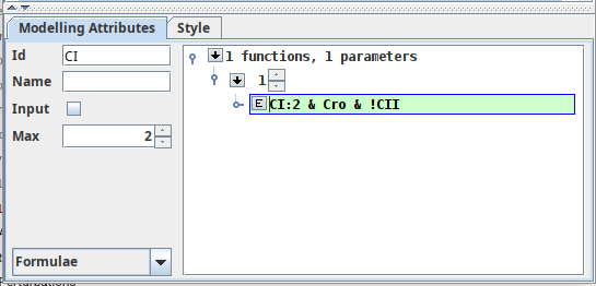
The logical function panel, showing the definition of one logical function at target 1.
To define a new logical function, select the Down arrow, specify a target value for the function, and select subsequent Down arrow.
You can then press the E button to start editing the logical function (line color changes to green).
After insertion of the logical function press Enter to validate the expression and automatically create the corresponding logical parameters.
The parser for logical functions accepts the logical AND and OR with the symbols & and |, respectively. Additionally, you can add parentheses to prioritize logical operations.
Annotations
Annotations can be attached to the different components of the regulatory graph:
- the graph itself,
- components,
- interactions.
An annotation is composed of a textual comment and a numbered list of URIs,
which can be opened using the [i] buttons on the left side.
The annotation panel
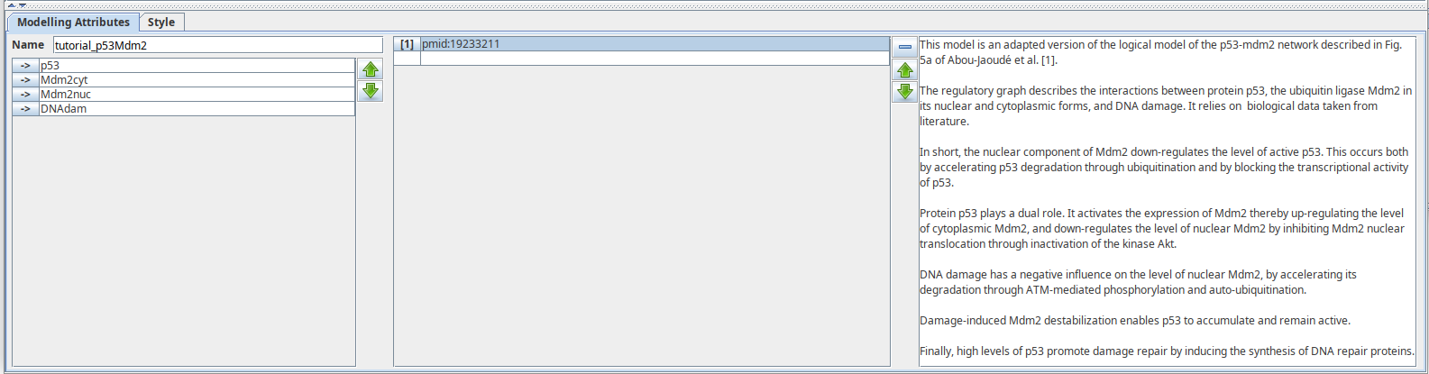
The same Annotation panel is used for all elements
supporting notes. This screenshot shows the graph annotations, available when the selection is empty.
Some shortcuts are provided for linking to entries in online databases.
For example, pubmed:19426782 will open http://www.ncbi.nlm.nih.gov/pubmed/19426782.
This relies on the identifiers.org webservice.
LRG modifications
Perturbations
GINsim facilitates the definition of perturbations to define small changes to the regulation of components in regulatory graphs. A perturbation is a set of restrictions on the evolution of the activity level of one or several components.
Using Perturbations
Some tools, notably Simulation and Stable state search, include a perturbation selection panel to apply a perturbation before running.
Definition of Perturbations
Perturbation can be defined using the following configuration panel.
The panel appears upon activation of the configure button in the
perturbation selection panel.
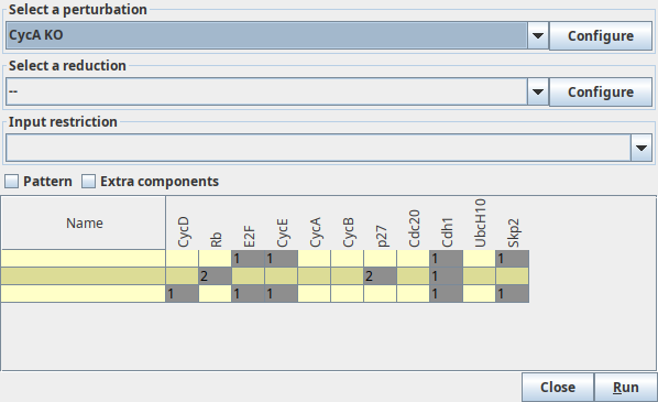
Perturbation definition panel
This edition panel considers two types of perturbations: simple perturbations which only affect the activity of a single component, and multiple perturbations which group together a list of simple perturbations.
Simple Perturbations
The perturbation definition panel appears on the top-right part of the dialog above
when no simple perturbation is selected, or when clicking the + button.
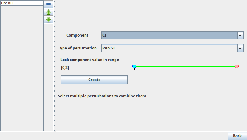
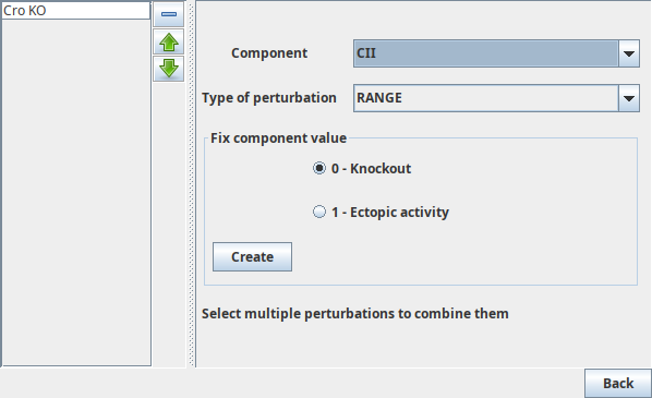
To create a perturbation, one must first select the affected component using the combobox.
The restriction configuration panel will then appear, and the perturbation can be added using the create button.
The activity level of Boolean components can be fixed at 0 or at 1,
corresponding to the definition of a knockdown or ectopic activity respectively.
Radio buttons allows to choose between these two possibilities.
Multi-valued components offer more possibilities, that can be configured using a range slider. Their activity level will be restricted in the selected range, or completely fixed if the range corresponds to a single value.
Perturbation creation panels
TODO: add multivalued figure figures/mvaluedperturbation.png
This enables the definition of simple perturbations where the activity level of a component is restricted to the selected value(s).
Info
The definition of more subtle perturbations (conditional knockouts...) still requires the modifications of the logical parameters. We plan to add convenient means to define other types of perturbations in the future.
Info
Simple perturbations cannot be duplicated: when trying to add a simple perturbation that is already defined, nothing will happen.
Multiple Perturbations
The bottom part of the panel lists multiple perturbations. Multiple perturbations can be created by selecting several simple perturbation and clicking the button which appears in the information panel. These perturbations can then be ordered and deleted using the buttons on the right side.
Warning
Deleting a simple perturbation will also remove all the multiple perturbations using it.
Booleanization
GINsim enables the definition of multi-valued models where some components can have several increasing activity levels. However, some other analysis tools only consider Boolean (on/off) models. Model booleanization allows to convert multi-valued models into Boolean models by mapping each multivalued component on a group of Boolean variables. The resulting Boolean model generates the same dynamical behaviour as the original multivalued model.
bioLQM uses the mapping originally proposed by van Ham, in which a component
associated with the maximal value m will be mapped on m Boolean components.
For example, a component taking the values 0`,1,2, and3will be
encoded as000,100,110, and111``.
The booleanization introduces many non-admissible states, which may require special care depending on the analysis applied on the booleanized model. This modifier makes sure that a simulation which start with an admissible state will not explore non-admissible states. It also prevents the introduction of non-admissible attractors by making sure that at least one admissible state is reachable from any non-admissible.
Usage
Exporting a multivalued model to a format limited to Boolean components triggers an implicit Booleanization step.
This booleanization step can also be performed explicitely using the booleanization tool in the Actions menu.
Availability and further reading
This method was implemented in GINsim 3.0. The backend is implemented in the bioLQM toolkit, enabling its programmatic use.
Model reversal
The model reversal tool constructs a model in which the asynchronous successors of a state correspond to its predecessors in the original model.
Multivalued models are supported through model booleanization, with some further transformations to prevent the introduction of non-admissible successor states.
Usage
The model reversal tool is available in the Actions menu.
Availability and further reading
This method was implemented in GINsim 3.0.
The backend is implemented in BioLQM <http://colomoto.org/biolqm>_,
enabling its programmatic use.
Model reduction
The reduction of regulatory graphs allows to extract a "simplified" regulatory graph where a set of components are hidden. To keep a consistent dynamical behaviour, the logical rules associated with the targets of each hidden component account for the (indirect) effects of its regulators. This construction of reduced models preserves crucial dynamical properties of the original model, including stable states and more complex attractors. Furthermore, the relationship between the attractor configuration of the original model and those of reduced models is formally established.
Usage
The reduction tool is available in the Actions menu. It open a
configuration dialog in which the user can select the components
that will be hidden. Several configuration strategies can be defined.
Running the tool leads to the construction of a reduced model where
the selected components have been removed.
Some reductions are not possible (an auto-regulated component cannot be hidden using this method), if a reduction fails, GINsim will show an error message, listing the components that could not be hidden and proposing to continue with the result of the partial reduction.
Note that in some cases, the reduction may only be possible in a precise order (but the result does not change with the order). When blocked, GINsim will try alternate orders for the remaining components, but not for the components which have already been succesfully reduced. In such cases, it may be necessary to provide the list of components to reduce in several steps to force the use of the correct order.
Output stripping
Outputs are components which do not regulate others. As such, these
components have no impact on the attractors that will be reached in
a simulation. These output components can be automatically removed
when performing a simulation or some other actions on a model.
To instruct GINsim to remove outputs, use the strip outputs
checkbox next to the perturbation selection box.
Script mode
The reduction tool can also be used in script mode. It then relies on a previously defined reduction strategy.
Availability and further reading
This method was implemented in GINsim 2.4 (see 3). The support for output stripping was added in GINsim 3.0 (see 5).
Model dynamics and properties
State transition graphs
A State Transition Graph (STG) is a directed graph representing the dynamical behaviour of a Logical Regulatory Graph. Nodes of this graph represent possible states of the model, assigning a value to each component. Arcs of the STG represent transitions from one state to another (i.e. change of value for one or several components).
For a more formal definition see 3.
Simulation
Once a regulatory model has been defined, a simulation can be launched
through the Run Simulation option of the Tools menu.
This option triggers a dialog box allowing to choose simulation settings.
Simulation settings
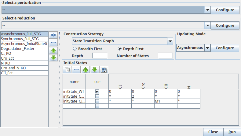
This dialog box allows to configure and run the simulation.
This dialog box allows to define simulation settings. The top part of the dialog box enables the definition of transformations to apply to the regulatory graph before the simulation. The left part of the dialog box enables to manage (select, add or remove) simulations settings. The right part of the dialog box enables the definition of the current simulation setting.
Initial states
Named groups of states can be defined for the regulatory graph and used for example as starting point for the Simulation.
Each row of the table corresponds to a set of states, where activity levels are specified for each component in the corresponding table cell. Each component can use all of its possible levels (denoted by a star ("*")), a single level or any subset of levels, separated by semicolons (;). Intervals can also be defined using a dash ("0-2" denotes all levels from 0 to 2, included). The special value "m" denotes the maximal level of the component. For example, "0;2-4" means "0 or values between 2 and 4" and is identical to "0;2;3;4". "1-m" means "any activity (from 1 to the max)". The default, denoted by a "*", covers all possible values (it is thus the same as "0-m").
Initial states can be reordered, deleted and duplicated using the buttons on top of the table.
Hint
A value can be entered in many cells at once using multiple selection.
Configure the simulation
The top part of the simulation dialog enables the selection of a perturbation
to be applied to the regulatory graph before running the simulation. The associated Configure
button will show the :doc:perturbation definition panel.
The bottom part of the dialog box is dedicated to the definition of
:doc:initial_states of the simulation.
Each row defines a single state or a group of states, and the checkboxes allow
to select the states used for the simulation. If no row is selected, all possible
states are considered, generating a complete state transition graph.
In a given state of the system, one or several genes are called to update their values. When several changes are pending, different construction strategies lead to different successor states and thus to different state transition graphs. GINsim implements the classical synchronous and asynchronous updating, and enables the definition of ad hoc strategies using priority classes. These updating modes are described in detail in their documentation.
Simulation settings are saved and restored as associated data in ZGINML files.
Running simulations with perturbation
Warning
I cannot reproduce the same graphics. The legend of the figure below seems not sufficient for me to reproduce.
Perturbation simulation result
Result of an asynchronous simulation, where the expression level for Cro has been blocked at 1. The state transition graph is the same as the original asynchronous one, but all transitions where Cro leaves this value have been suppressed. This state transition graph is now composed of two disconnected parts, with a new stable state.
The "strip output" checkbox next to the perturbation selector enables to activate automatic removal of all output components from the simulation. Their value can be retrieved on demand when browsing the resulting State Transition Graph. See the reduction section for more details.
The "Construction Strategy" panel enables the selection of the type of graph computed by the simulation (the classical State Transition Graph, or the more compact Hierarchical Transition Graph).
State Transition Graphs can be computed breadth-first or depth-first. Both options lead to the same result, unless the simulation is interrupted by a size limit (see below).
Depth and size limitations
An option is also offered to limit the search depth and/or the total number of states generated in a simulation.
Warning
When considering several initial states (or the full STG), some of them can be reached while running the simulation from an other state. In this case, no new search will be triggered for them and the depth counter will not be reinitialised (i.e. the depth limit for these initial states will be shorter).
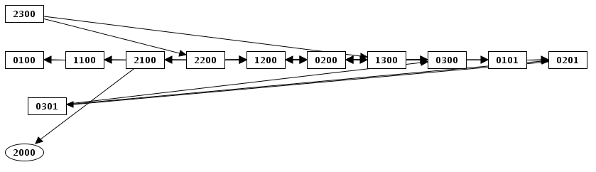
Limitation of the depth in the case of a depth first construction
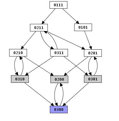
State transition graph with all reachable states from the state "0111". The same simulation with a depth limit set to 2 keeps only the initial state and the nodes at a distance of two or less (i.e. the six white states).
The limit on the total number of states apply to all simulation modes. Under the asynchronous assumption, this limit has slightly different effects on depth first and breadth first search.
Limitation of STG size
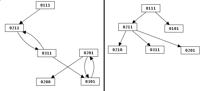
Limitation of the size (depth first and breadth first search construction). The limit on the total number of nodes has different effects on depth first and breadth first state transition graphs. These examples show the graph of the figure above [TODO: figure link] limited to 6 states. The first state transition graph was obtained using the depth first construction, whereas the second results from the breadth first one.
Running the simulation
While the simulation is running, the bottom left corner indicates
the size of the generated state transition graph. The simulation
can be interrupted, using the Cancel button, without loosing
the calculated part of the state transition graph.
At the end of a simulation, several options are available to save, display or analyse the resulting state transition graph (see ).
Updating modes
In a given state of the system, one or several genes are called to update their values. When several changes are pending, different construction strategies lead to different successor states and thus to different state transition graphs.
Synchronous mode
In this mode, all updating calls are performed simultaneously. This simplification may generate artefacts in the state transition graph.
Each state has then at most one successor state, which encompasses fully updated gene levels.
Asynchronous mode
In this mode, all changes are performed independantly. It will generate a state transition graph taking into account any possible trajectories. This mode is chosen by default.
A given state may have several successor states, each of them corresponding to a single updating of one gene level.
In this mode, the graph transition state can be generated "depth first" or
"breadth first". The same state transition graph will be built, except if
interrupted (for illustration, see :doc:depth and size limitation).
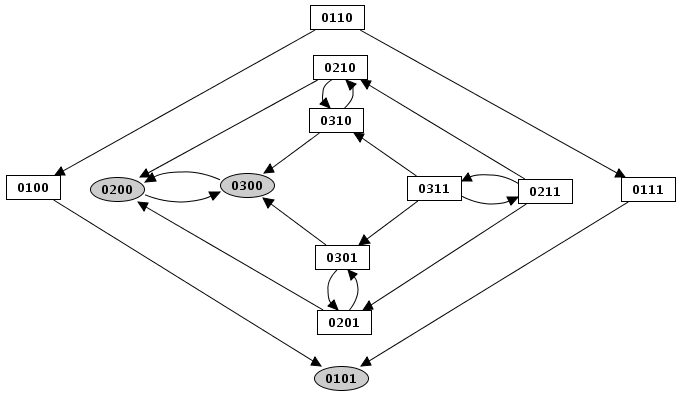
Construction strategy: synchronous versus asynchronous
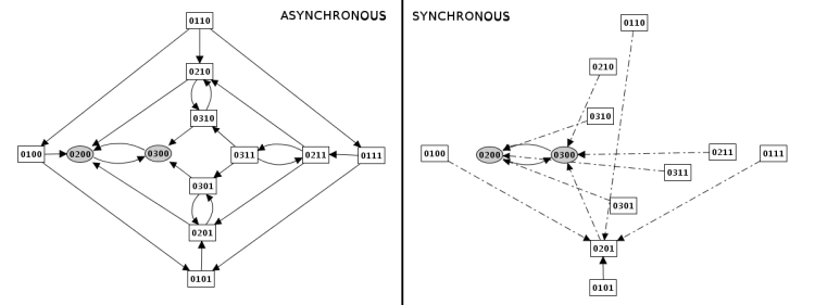
Samples of simulation results for the lambda4 model, applying asynchronous and synchronous strategies to the same initial states (all states where C1=0 and Cro>0). Dotted arcs denote multiple, simultaneous transitions.
Priority classes
This strategy allows the user to group components into different classes, and to assign a priority level to each of these classes. In case of concurrent transition calls, GINsim first updates the gene(s) belonging to the class with the highest ranking. For each class, the user can further specify the desired updating assumption, which then determines the treatment of concurrent transition calls inside that class. When several classes have the same ranking, concurrent transitions are treated under an asynchronous assumption (no priority).
The creation of a new configuration, using the leftmost "+" button, starts wth some predefined settings:
- The definition of a single class contaning all components, equivalent to the (a)synchronous updating.
- The definition of a fully-ordered updating using a separate class for each component.
- The separation of the increasing and decreasing transition of each components for more fine-grained configurations.
The left part of the configuration dialog box shows a list of priority classes (see figure below). The name of a class can be edited and a checkbox allows to change its internal mode from asynchronous (unchecked) to synchronous (checked). Buttons enable to add (+), delete (X), order (using the arrows) and group/ungroup priority classes.
The central column lists transitions that belong to the currently selected
class, while the column on the right displays all other transitions (i.e. belonging to
other classes). To add transitions to the selected class, choose them in the
right list an click on the "<<" button. The >> button removes the
transition selected in the central list from the current class and add them to
the next class in the list (to the first class when the last one is selected).
When multiple classes are selected, they can be assigned the same rank. Multiple classes with the same rank are treated asynchronously: if all classes are asynchronous, it is thus equivalent to a single larger class, but it allows the definition of asynchronous update of multiple synchronous classes as well.
Definition of Priority classes
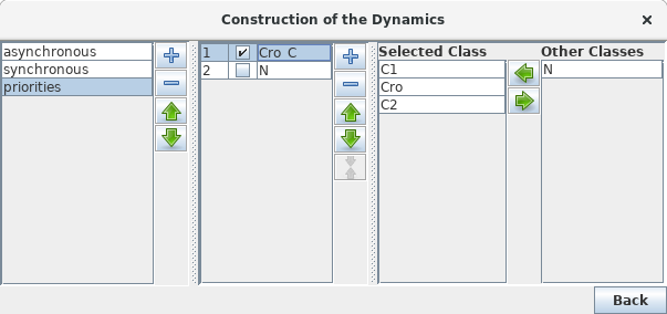
Priority Class: example result
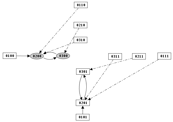
Example of simulation by priority classes. Two priority classes have been created. The highest ranked one is synchronous and contains C1, C2 and Cro. The other class contains only N. The resulting state transition graph is splited into two parts: N expressed versus N not expressed.
Hierarchical Transition Graphs
The Hierarchical Transition Graphs (HTG) is an acyclic graph, which provides a compact representation of the State Transition Graph. It improves on the graph of the Strongly Connected Components by merging linear chains of states (in addition to cycles) into single nodes.
More information on this graph is available in Berenguier et al6.
Analyses / Functionalities
Strongly Connected Components graph
A Strongly Connected Component (SCC) in a graph is a maximal subgraph such that all its components are strongly connected. Each SCC can be either a single node or a set of intertwined cycles of the original graph. The SCC graph is a derived graph in which each node represents one of the SCC of the original graph. This acyclic graph provides a simplified representation of the organisation of the original graph. This graph is thus often much more compact.
In GINsim, the graph of the Strongly Connected Components (SCC graph) is often used to provide a better understanding of the organisation of the attractors in a State Transition Graph.
Construct an SCC graph
The computation of the SCC graph can be launched through the Construct SCC graph
option of the Tools menu.
Note that GINsim also provides the Hierarchical Transition Graph dedicated to this problem.
Strongly Connected Components graph
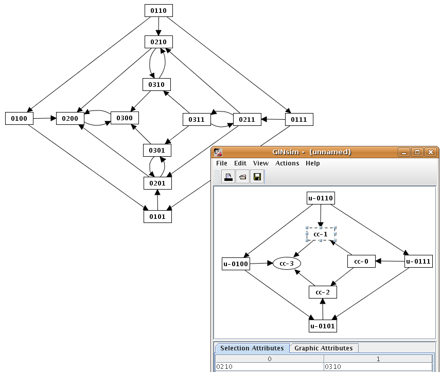
Example of Strongly Connected Component Graph (bottom right) and the corresponding state transition graph (top left).
The Selection Attribute tab in the bottom panel shows the content of the selected SCC (i.e. the list of nodes in the original graph).
Note that while the Construct SCC Graph tool is often applied to State Transition Graph, it can
also be applied to Regulatory Graphs (or more formally to any type of graphs).
Extract from SCC graph
After computing the SCC graph, another tool allows to recover the subgraph of the original graph corresponding to the selected nodes in the SCC graph.
To use it, select some nodes in a SCC graph and run the Extract subgraph
action from the Graph menu.
This tool will open the original graph, and apply a filter to only keep the selected parts. To work properly it thus requires that the original graph had been saved to a file, and that the association between the SCC graph and the original graph (maintained by GINsim transparently) is still valid.
Stable state search
This tool allows the analytic (i.e. without running a simulation) determination of stable states of the model. All stable states are determined, regardless of their reachability7.
This tool allows the analytic (i.e. without running a simulation) determination of trapspaces of the model. These trapspaces contain the stable states, as well as an approximation for complex attractors.
Usage
The stable state identification tool is available from the Compute stable states option of the Tools menu.
The stable states dialog box allows to run the analysis after the optional
selection of a perturbation. The result is shown in a table in the same dialog box, allowing to launch a novel analysis for another perturbation.
A "*" in the table denotes that each of the values of this component gives rise to a stable state (or several if another "*" appears in the same row).
Stable states search
The stable states dialog box, showing the result of the analysis.
Availability
Stable state search was first implemented in GINsim 2.3. The implementation is now part of the bioLQM toolkit.
Trapspace search
This tool allows the analytic (i.e. without running a simulation) determination of trapspaces of the model. These trapspaces contain the stable states, as well as an approximation for complex attractors cite Klarner2014.
Usage
This tool is available from the Trapspace identification option of the Tools menu.
The trapspace dialog box

The trapspace dialog box, showing the result of the analysis.
Availability
Trapspace identification was first implemented in GINsim 3.0, relying on the bioLQM toolkit.
Circuit analysis
Regulatory circuits play crucial roles in the dynamical behaviour of a system. Indeed, positive circuits are required for the existence of several attractors, whereas negative circuits may generate cyclic attractors4.
Many regulatory graphs currently under study contain a large number of circuits, but a relatively small number of them often plays a more important role. In 7, we describe a method to compute a functionality context for all circuits, to determine which circuits are more likely to affect the attractor configuration of the system.
Note that the functionality contexts identified here give the conditions on the immediate regulators of the circuits under which it is fully effective. These conditions may be impossible to maintain according to the dynamical rules of the model, especially in the case of model perturbations.
Usage
The Circuits Functionality entry of the Action menu opens the circuit
analysis dialog. This dialog provides an interface to lookup all circuits in the
regulatory graph or a subset of circuits matching some filtering rules (length,
involved components).
Select regulatory circuits for analysis
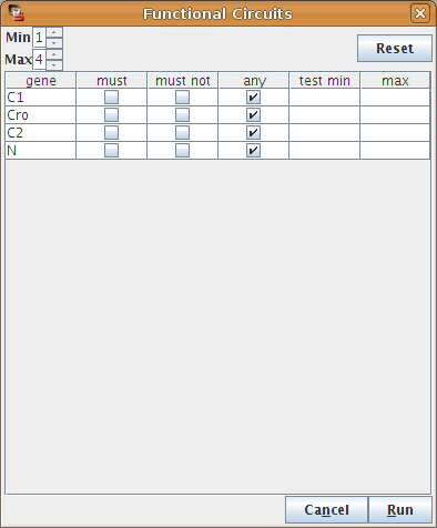
A first dialog allows to select which circuits will be analysed, by specifying constraints on the length of the circuits or on the involved actors. By default all circuits are considered.
The dialog then allows to analyse the selected circuits, it will then show the circuit for which a functionality context was found. The analysis can be repeated for various perturbations.
Result of the functionality analysis
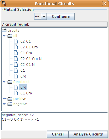
When the analysis is completed, the dialog classifies the selected circuits, according to their computed sign. When a circuit is selected, its functionality context is shown at the bottom of the dialog box.
Availability
Circuit analysis was implemented in GINsim 2.3.
Graph layouts
The "Layout submenu of the "View" menu provides some tools to place graph components automatically. These layout tools are mostly useful for graphs computed by GINsim, such as state transition graphs. Note that GINsim only offers very simple layout tools. For complex cases, dedicated tools such as graphviz or cytoscape can provide much better results. The following layouts are available:
Level layout
Nodes are placed on rows, nodes without any incoming arc being placed at the top and nodes without any outgoing arc at the bottom.
Level layout example
Ring layout
Nodes are placed on three concentric rings, source nodes at the center, terminal nodes at the periphery.
Ring layout example
STG layouts
State transition graphs have additional layout methods which place components on a grid based on the activity levels.
Formats (imports/exports)
GINsim format
The Z-GINML format (also denoted extended save), is a zip archive containing a ginml file along with companion files to store associated data, especially initial states, perturbations, and simulation parameters. More generally, each plugin can provide a parser and file writer to store its associated data in a Z-GINML file.
The GINML format is an extension of the GXL (Graph eXchange Language) format. This extension comprises new attributes and subelements for elements node and edge, and an additional element called parameter.
element node a new attribute basevalue corresponds to the "base level of expression" of the corresponding component (default value 0). In other words, it is the value of the logical parameter corresponding to the case where none of the incoming interactions is functional. New subelements within a node:
a list of elements parameter corresponding to the user defined logical parameters for this node
an element intdefining the maximum level of expression of this node
element edge a new attribute sign which gives the sign of the interaction (positive for an activation, negative for a repression, otherwise unknown) one or two subelements int (level or interval letting the interaction functional) element parameter, is empty and has two attributes : attribute idActiveInteractions gives the "name" of the parameter. It is the list of the functional interactions exerted upon the considered node, attribute val is the value of the logical parameter.
See the GINML's dtd or in pdf format.
See also the GINML description of the gap-gene network case A, or in pdf format.
(TODO: described stored associated data)
Some companion data can be associated to the graphs to store the configuration of various tools. Some of this extra data can be shared between several tools. This extra data is stored in its own entry inside ZGINML files.
Export graph view
The graph view can be exported as an image in the PNG format. This export considers only the visual appearance of the graph, and can thus be applied to all types of graph in GINsim.
The view can also be exported in the Scalable Vector Graphic (SVG) format. Tools like Inkscape, can then be used to display, modify and export SVG files to virtually any image format.
Export graph structure
The following exports consider only the graph structure, and can thus be applied to all types of graph in GINsim.
The graph structure can be exported for use in dedicated graph visualization software, which can handle some graphs considered as too large for viewing in GINsim directly. These exports only consider the graph structure (graphical attributes are lost). The following formats are supported:
Graphviz
Files in the DOT language can be opened using the graph visualization software Graphviz.
BioLayout
Biolayout, is a graph visualization software focussing on biological networks.
Cytoscape
Cytoscape, is also used for the analysis of biological networks. While GINsim can export regulatory graphs for cytoscape, this format is not yet available for other types of graphs.
NuSMV export
The dynamics of logical regulatory graphs can be described using a NuSMV specification. In GINsim, this specification is created through an export functionality capable of generating a symbolic description of the logical model specified in GINsim.
Additionally, it is capable of describing different updating policies for the generation of the successors, such as synchronous, asynchronous and priority classes.
Finally, it tries to address the space problem of the state representation by annotating the information regarding the input variables on edges instead of states (making use of ARCTL), and by (optionally) defining output variables as simple macro functions.
Symbolic representation
Each variable is declared under the VAR section together with
the corresponding range of values (domain). The order of the declaration of
variables is of extreme importance since it influences the construction of the
internal BDD representing the whole dynamics.
The initialization of a set of variables is performed by using the
INIT keyword followed by an assignment of a value to a given variable.
Alternatively, a macro can be defined with a conjunction of variable valuations
and simply use the macro name with the INIT keyword.
The rules concerning the computation of the target value of a given variable
are described under the ASSIGN section, using the
next(Var) := ...; form.
The computation of the focal point is declared under the DEFINE
section, where the actual logical rules referencing all the regulatory
components are declared.
In this section it is also declared all the macros to be used in the property specifications, such as weak and strong stable states, the list of initial conditions defined by the user, or the output variables which (if specified) do not participate in the state characterization.
Updating policies
In this export, all of the possible updating policies synchronous/asynchronous are considered as being special cases of the priority classes:
- Asynchronous updating is represented as having one priority class per variable ([VarA] [VarB] ... [VarZ]), with the restriction of a single class update per successor.
- Synchronous updating is represented as having one single priority class containing all of the variables ([VarA VarB ... VarZ]), where all of the variables in the class are called to change their value in the (single) successor.
State representation
There are three main types of variables characterizing a state:
state variables, which are declared under the VAR section;
output variables, which (if specified by the "Strip outputs" option) are declared
as macros under the DEFINE section;
and the input variables, which are declared under the IVAR section.
State variables are the ones characterizing an internal state in NuSMV, so, whenever one of the state variables is called to change, a new successor is (might be) created. Output variables are the ones that are not critical for the state characterization, and whose values can be computed through state variables alone. Output variables can still be referenced with a temporal operator in a property specification though. Input variables are always projected over transitions rather then the state. Between a state and its successor, a transition contains all the valid input valuations, i.e., if a given input valuation does not permit to follow a given transition is will be not represented over that transition.
Macros representing state restrictions
The NuSMV export will always automatically compute the model stable states and insert them in the NuSMV model description. Every stableState is either a weakSS or a strongSS, and each one of these can be composed by several ones, depending on the model. The user, can then use each of these macro names for the specification of properties, from a general one stableState to a more specific one strongSS.
Additionally, when exporting a model, the user can define and select state restrictions on the internal components or on the input components. Only the ones that are checked will be written on the NuSMV specification. Similarly, the names given to each of these state restrictions will correspond to macro names which can be used in the specification of properties.
Temporal logic property specification
This NuSMV specification of the logical model, does not include any property specifications. It is up to the user to encode them at the end of the NuSMV specification file. Again, in any given property, the user can always use the stableState or the initialStateList macros previously defined. In order to aid the user in such task, the following example reachability properties are added, as comments, at the end of each file.
--------------------------------------------------
-- Reachability Properties using VARYING INPUTS --
-- i.e. there is NO CONTROL on the input change at each transition
--
-- 1. Between an initial state (pattern) and a stable state (pattern)
--   a. Existence of at least one path connecting two state patterns
-- INIT initState;
-- SPEC EF ( stableState );
--   b. Existence of all the paths connecting two state patterns
-- INIT initState;
-- SPEC AF ( stableState );
--
-- 2. Between all the weak/strong stable states
-- INIT weakSS1;
--  SPEC EF ( weakSS2 );
--  ...
--  SPEC EF ( weakSSn );
--------------------------------------------------
-- Reachability Properties using FIXED INPUTS --
-- i.e. a VALUE RESTRICTION can be forced at each transition
--
-- 1. Between an initial state (pattern) and a stable state (pattern)
--   a. Existence of at least one path connecting two state patterns
-- INIT initState; SPEC EAF ( inpVar1=0 & inpVar3=1 )( stableState );
--   b. Existence of all the paths
-- INIT initState; SPEC AAF ( inpVar1=0 & inpVar3=1 )( stableState );
--
-- 2. Testing input combinations
-- INIT weakSS1;
--  SPEC EAF ( inpVar1=0 & inpVar2=0 )( weakSS2 );
--  SPEC EAF ( inpVar1=0 & inpVar2=1 )( weakSS2 );
--  SPEC EAF ( inpVar1=1 & inpVar2=0 )( weakSS2 );
--  SPEC EAF ( inpVar1=1 & inpVar2=1 )( weakSS2 );
--  ...
Availability and further reading
This export was implemented in GINsim 3.0. Further information is available in 8.
Petri net export
Regulatory graphs can be exported into discrete Petri net using the rewriting method described in 9.
In the "File -> Export" menu, a "Petri Net" submenu allows to choose one of three supported Petri net representations: INA, PNML and APNN. Choosing any of these representations, opens a configuration dialog box which presents a list of options to be considered in the export. These include modifications such as model perturbations or reductions, or the definition of a set of initial states.
The Petri Net export dialog
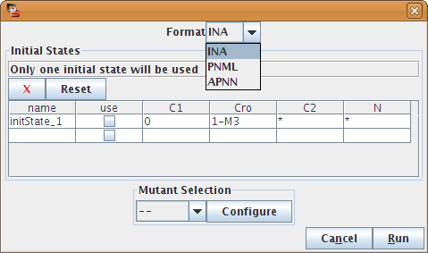
The Petri Net export dialog box allows to select the export format, the initial markup and the mutant to apply before exporting. The initial markup can be generated from an existing initial state of the model (modifications made in this dialog are also applied to the simulation settings); only the first selected state is used.
TODO: update figure!
-
Hidde de Jong. Modeling and simulation of genetic regulatory systems: a literature review. Journal of Computational Biology, 9(1):67–103, January 2002. doi:10.1089/10665270252833208. ↩
-
Claudine Chaouiya, Aurélien Naldi, and Denis Thieffry. Logical Modelling of Gene Regulatory Networks with GINsim, pages 463–479. Springer New York, October 2012. doi:10.1007/978-1-61779-361-5_23. ↩
-
Aurélien Naldi, Elisabeth Remy, Denis Thieffry, and Claudine Chaouiya. Dynamically consistent reduction of logical regulatory graphs. Theoretical Computer Science, 412(21):2207–2218, May 2011. doi:10.1016/j.tcs.2010.10.021. ↩↩↩
-
D. Thieffry. Dynamical roles of biological regulatory circuits. Briefings in Bioinformatics, 8(4):220–225, March 2007. doi:10.1093/bib/bbm028. ↩↩
-
Aurélien Naldi, Pedro T. Monteiro, and Claudine Chaouiya. Efficient Handling of Large Signalling-Regulatory Networks by Focusing on Their Core Control, pages 288–306. Springer Berlin Heidelberg, 2012. doi:10.1007/978-3-642-33636-2_17. ↩
-
D. Bérenguier, C. Chaouiya, P. T. Monteiro, A. Naldi, E. Remy, D. Thieffry, and L. Tichit. Dynamical modeling and analysis of large cellular regulatory networks. Chaos: An Interdisciplinary Journal of Nonlinear Science, June 2013. doi:10.1063/1.4809783. ↩
-
Aurélien Naldi, Denis Thieffry, and Claudine Chaouiya. Decision Diagrams for the Representation and Analysis of Logical Models of Genetic Networks, pages 233–247. Springer Berlin Heidelberg, 2007. doi:10.1007/978-3-540-75140-3_16. ↩↩
-
Pedro T. Monteiro and Claudine Chaouiya. Efficient Verification for Logical Models of Regulatory Networks, pages 259–267. Springer Berlin Heidelberg, 2012. doi:10.1007/978-3-642-28839-5_30. ↩
-
Claudine Chaouiya, Elisabeth Remy, and Denis Thieffry. Qualitative Petri Net Modelling of Genetic Networks, pages 95–112. Springer Berlin Heidelberg, 2006. doi:10.1007/11880646_5. ↩